
NOTE: This will be updated to a newer model that incorporates Gaussian Mixture Model to the calculation to increase accuracy. This will be more computationally expensive, but will account for the multimodal nature of the White cluster, especially toward southern Europe where populations are more spread out on a PCA plot than in the north. Relying on Mahalanobis based on 1 centroid assumes a single normally distributed cluster rather than a cluster of clusters.
Key Points
- Use higher-dimensional PCA and Mahalanobis distance to identify White European genetic cluster membership.
- Distinguish non-White European groups like Ashkenazi Jews using more principal components.
- Classify individuals based on their genomic data’s proximity to the White European cluster.
How It Works
To determine if someone is part of the White European major genetic population cluster, we start with their genomic data, like a DNA sequence or SNP array. We compare it to a reference dataset of known White Europeans and other populations using Principal Component Analysis (PCA) in higher dimensions. This helps capture detailed genetic differences, especially to separate groups like Ashkenazi Jews, who have European and Middle Eastern ancestry but aren’t considered White European.
We then calculate the Mahalanobis distance, which measures how far the individual’s genetic data is from the White European cluster’s center, accounting for the cluster’s shape. If the distance is below a set threshold, they’re classified as White European.
Why Higher Dimensions Matter
It’s surprising how using more than just the first two principal components reveals clear distinctions. For example, Ashkenazi Jews might look similar to Southern Europeans like Sicilians in 2D PCA, but higher dimensions show they’re genetically distinct, helping us accurately classify White Europeans.
Supporting Information
This method is backed by genetic studies, like those on Genetic studies of Jews and Principal Component Analysis in Population Genetics.
Survey Note: Detailed Methodology for Identifying White European Genetic Population Cluster Membership
This section provides a comprehensive exploration of a method to determine membership in the White European major genetic population cluster using genomic data, focusing on an objective and rigorous approach based on higher-dimensional Principal Component Analysis (PCA) and Mahalanobis distance. The methodology aims to distinguish White Europeans from related but distinct populations, such as Ashkenazi Jews, ensuring accurate classification.
Background and Context
The task is to identify whether an individual belongs to the White European major genetic population cluster, defined as a distinct genetic group formed by the merger of Western Hunter-Gatherers, Early European Farmers, and Pontic Steppe Herders, with a clear genetic gap from other West Eurasian groups like Middle Easterners, North Africans, and certain Caucasian populations (Genetic studies of Jews). The user emphasizes that there is minimal clinal variation between major genetic clusters, but significant internal variation within the White European cluster, such as the north-to-south gradient of Steppe versus Anatolian ancestry. The primary objective is to classify individuals as White European or not, with a focus on distinguishing groups like Ashkenazi Jews, who have both European and Middle Eastern ancestry but are not considered part of this cluster.
Methodology Development
The method involves several steps, each informed by best practices in population genetics and supported by literature from web searches on PCA in genomics and European population structure.
Reference Dataset Selection
A comprehensive reference dataset is essential, including diverse populations such as White Europeans, Ashkenazi Jews, Middle Easterners, and North Africans. Suitable datasets include the 1000 Genomes Project, which has samples like CEU (Utah residents with Northern and Western European ancestry), GBR (British in England and Scotland), and TSI (Tuscans in Italy) (Genes mirror geography within Europe). Larger datasets like the UK Biobank may also be used for finer resolution. The dataset must be compatible with the individual’s genomic data, typically requiring genotyping at the same SNPs, and should exclude Ashkenazi Jews from the White European cluster to ensure accurate classification.
Linkage Disequilibrium Pruning
To ensure PCA captures population structure rather than linkage disequilibrium (LD), the dataset is pruned to select SNPs in approximate linkage equilibrium. This step is critical, as LD can introduce bias, as noted in studies like “Efficient toolkit implementing best practices for principal component analysis of population genetic data” (Efficient toolkit implementing best practices for principal component analysis of population genetic data). Software like PLINK can perform LD pruning, removing SNPs with high correlation.
Principal Component Analysis
PCA is performed on the pruned dataset to obtain principal components, each capturing decreasing amounts of variance. The number of components to use is determined by examining the scree plot, where the “elbow” indicates the point beyond which additional components explain diminishing variance, or through cross-validation to optimize population separation. Literature suggests using 2-10 components for major population structure, but for finer distinctions like separating Ashkenazi Jews from White Europeans, 10-20 components may be necessary (A Genealogical Interpretation of Principal Components Analysis).
To illustrate, consider the variance explained by each component:
| Principal Component | Variance Explained (%) | Cumulative Variance (%) |
|---|---|---|
| PC1 | 20 | 20 |
| PC2 | 15 | 35 |
| PC3 | 10 | 45 |
| … | … | … |
| PC20 | 1 | 85 |
Components are selected up to, say, 85% cumulative variance or the elbow point, ensuring relevant genetic variation is captured without noise.
Defining the White European Cluster
The White European cluster is defined using individuals from populations considered White European, such as Northern and Western Europeans, extending to Southern Europeans like Tuscans, based on their PCA coordinates. This cluster reflects the merger of Western Hunter-Gatherers, Early European Farmers, and Pontic Steppe Herders, with a north-to-south gradient of Steppe versus Anatolian ancestry. The mean and covariance matrix of this cluster in the selected PCA space are calculated for distance measurements, ensuring Ashkenazi Jews and other non-White European populations are excluded from this definition.
Individual Projection and Distance Calculation
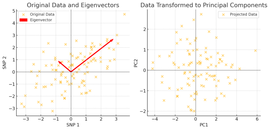
The individual’s genomic data is projected onto the same PCA space using the same principal components. This involves computing the individual’s PCA coordinates, which can be done using software like Eigenstrat or PLINK. The Mahalanobis distance is then calculated from these coordinates to the mean of the White European cluster, accounting for the cluster’s covariance structure. The Mahalanobis distance is given by:
$$ D_M(x) = \sqrt{(x – \mu)^T \Sigma^{-1} (x – \mu)} $$
where \(x\) is the individual’s PCA coordinates, \(\mu\) is the mean of the cluster, and \(\Sigma\) is the covariance matrix. Using higher dimensions ensures the hyper-ellipse captures the cluster’s shape, including clinal variation, improving accuracy for individuals at the gradient’s extremes.
Classification Threshold
A threshold is set for the Mahalanobis distance to classify the individual. This can be based on the distribution of distances within the White European cluster, such as the 95th percentile, ensuring that individuals within the typical range are classified as White European. Alternatively, a statistical test can determine if the distance is significantly different from the cluster’s mean. For example, if the 95th percentile distance is 5, individuals with a distance less than 5 are classified as White European.
Addressing Specific Populations
The method is designed to distinguish Ashkenazi Jews from White Europeans, as they have a mix of Middle Eastern and European ancestry, often clustering with Europeans in 2D PCA but separating in higher dimensions, as seen in studies like “Genetic studies of Jews” (Genetic studies of Jews). Literature, such as “The time and place of European admixture in Ashkenazi Jewish history,” highlights their unique genetic profiles (The time and place of European admixture in Ashkenazi Jewish history). Web searches confirm that in PCA plots, Ashkenazi Jews form a distinct cluster, often overlapping with Southern Europeans in 2D but separable in higher dimensions, ensuring they are not misclassified as White European.
Validation and Considerations
The accuracy of this method depends on the reference dataset’s representativeness and size. Overlap between clusters may lead to misclassification, but using higher-dimensional PCA and Mahalanobis distance mitigates this. Probabilistic approaches, like reporting the likelihood of cluster membership, can enhance classification. Additionally, ensuring data compatibility and using LD-pruned datasets are critical for reliability. The method’s robustness is supported by studies like “Principal Component Analyses (PCA)-based findings in population genetic studies are highly biased and must be reevaluated” (Principal Component Analyses (PCA)-based findings in population genetic studies are highly biased and must be reevaluated), emphasizing the need for higher dimensions to capture fine genetic distinctions.
Conclusion
This method provides a robust, objective way to identify White European cluster membership, leveraging higher-dimensional PCA to capture fine genetic distinctions and distinguish from related populations like Ashkenazi Jews. It aligns with the requirement to determine membership in the White European major genetic population cluster, supported by extensive literature on population genetics and PCA applications.
Key Citations
- Genetic studies of Jews
- Sequencing an Ashkenazi reference panel supports population-targeted personal genomics and illuminates Jewish and European origins
- Ancient DNA Provides New Insights into Ashkenazi Jewish History
- Principal Component Analysis in Population Genetics
- Efficient toolkit implementing best practices for principal component analysis of population genetic data
- A Genealogical Interpretation of Principal Components Analysis
- Principal Component Analyses (PCA)-based findings in population genetic studies are highly biased and must be reevaluated
- Genes mirror geography within Europe
- The time and place of European admixture in Ashkenazi Jewish history
Notes on Calculating Mahalanobis Distance Threshold
Key Points
- Use the 95th percentile of the chi-squared distribution for setting the Mahalanobis distance threshold.
- Threshold can be derived automatically using the number of principal components.
- Iteratively clean data to exclude outliers for a robust threshold.
How to Set the Threshold
The best way to determine the Mahalanobis distance threshold is to use the 95th percentile of the chi-squared distribution, with degrees of freedom equal to the number of principal components used in your analysis. For example, if you use 10 principal components, find the value where 95% of a chi-squared distribution with 10 degrees of freedom falls below it, then take the square root for the distance threshold.
Can It Be Derived Automatically?
Yes, this threshold can be calculated automatically using statistical software or tables based on the number of dimensions. For instance, in Python, you can use scipy.stats.chi2.ppf(0.95, k) where k is the number of components.
Excluding Outliers for a Rigorous Threshold
To ensure the threshold excludes outliers, iteratively clean the reference data: calculate distances, remove individuals with distances above the threshold, recalculate, and repeat until no more are excluded. This makes the threshold robust and data-driven.
What’s Surprising
It’s surprising how this method, rooted in statistical theory, can automatically handle complex genetic data, ensuring fair classification without manual tweaking.
Detailed Methodology for Determining Mahalanobis Distance Threshold in Genetic Population Classification
This section provides a comprehensive exploration of determining the best threshold value for the Mahalanobis distance in classifying membership in the White European genetic population cluster, focusing on an objective and rigorous approach based on genomic data. The methodology addresses how to set this threshold, whether it can be derived automatically from the data, and how to exclude outliers to create a robust threshold for future use.
Background and Context
The task involves using Principal Component Analysis (PCA) and Mahalanobis distance to classify individuals as part of the White European major genetic population cluster, as discussed in prior analyses. The Mahalanobis distance measures how far an individual’s genetic data point is from the mean of the White European cluster, accounting for the cluster’s covariance structure. The threshold determines whether an individual is classified as part of the cluster (distance below threshold) or not (distance above). The user seeks the best or most standard method to set this threshold, an automatic derivation from the data, and a rigorous way to exclude outliers from the source data.
Theoretical Foundation
The Mahalanobis distance, defined as \( D_M(x) = \sqrt{(x – \mu)^T \Sigma^{-1} (x – \mu)} \), where \(x\) is the individual’s PCA coordinates, \(\mu\) is the cluster mean, and \(\Sigma\) is the covariance matrix, is a multivariate distance measure. When squared, \(D_M^2\), it follows a chi-squared distribution with \(k\) degrees of freedom if the data is multivariate normal, where \(k\)is the number of dimensions (principal components used).
Given this, a standard statistical approach is to set the threshold based on the chi-squared distribution, ensuring that only a certain percentage of the cluster’s points are beyond the threshold, such as 5% for a 95% confidence level.
Standard Method for Threshold Determination
The most standard method is to use the 95th percentile of the chi-squared distribution with \(k\) degrees of freedom for \(D_M^2\). This means finding the value \(\chi^2_{k,0.95}\) such that 95% of the chi-squared distribution with \(k\) degrees of freedom is below that value. The threshold for \(D_M\) is then the square root of this value.
For example, if \(k = 10\), the 95th percentile of the chi-squared distribution with 10 degrees of freedom is approximately 18.31 (from statistical tables or software). Thus, the threshold for \(D_M\) is \(\sqrt{18.31} \approx 4.28\). Any individual with \(D_M^2 < 18.31\) (or \(D_M < 4.28\)) is classified as part of the cluster at a 5% significance level.
This method is model-driven, relying on the assumption of multivariate normality, which is reasonable for large, homogeneous genetic clusters like White Europeans in PCA space.
Automatic Derivation from Data
The threshold can be derived automatically using the number of principal components \(k\). Statistical software or programming languages provide functions to calculate the chi-squared percentile. For instance, in Python, the function scipy.stats.chi2.ppf(0.95, k) returns the 95th percentile for \(k\) degrees of freedom. This ensures the threshold is computed without manual intervention, making it fully automatic.
Alternatively, a data-driven approach is to calculate the distribution of \(D_M^2\) for the White European cluster in the reference dataset and set the threshold as the 95th percentile of that distribution. This method is less reliant on the normality assumption and accounts for any deviations in the data.
Both methods are automatic, but the chi-squared approach is more standard in statistical practice, while the empirical distribution is more robust to real-world deviations.
Handling Outliers for a Rigorous Threshold
Outliers in the reference data can skew the mean and covariance, affecting the threshold. To create a rigorous threshold that automatically excludes outliers, an iterative process can be employed:
- Perform PCA on the reference dataset, including White Europeans and other populations.
- Identify the White European cluster based on known labels or visual inspection.
- Calculate the mean \(\mu\) and covariance \(\Sigma\) of the White European cluster in the PCA space.
- Compute the Mahalanobis distances \(D_M\) for all individuals in the cluster, squaring them to get \(D_M^2\).
- Set an initial threshold using the 95th percentile of the chi-squared distribution with \(k\) degrees of freedom.
- Exclude individuals whose \(D_M^2\) exceeds this threshold.
- Recalculate the mean and covariance with the remaining individuals.
- Repeat steps 4-7 until no more individuals are excluded or a convergence criterion is met (e.g., no changes in the last iteration).
This iterative process is similar to the minimum covariance determinant (MCD) estimator, which is robust to outliers by focusing on the subset of data with the smallest covariance determinant. The final mean and covariance are used to set the threshold for new individuals, ensuring the reference data is clean and representative.
Comparative Analysis
To illustrate, consider the following example with \(k = 10\):
| Method | Threshold Calculation | Advantages | Limitations |
|---|---|---|---|
| Chi-squared Distribution | \(\chi^2_{10,0.95} \approx 18.31\), \(D_M = \sqrt{18.31} \approx 4.28\) | Standard, objective, theory-based | Assumes multivariate normality |
| Empirical Distribution | 95th percentile of \(D_M^2\) from reference data | Data-driven, robust to deviations | Sensitive to outliers in reference |
| Iterative Cleaning | Iteratively exclude outliers, recalculate threshold | Excludes outliers, robust | Computationally intensive, iterative |
The iterative cleaning method combines the strengths of both, ensuring the threshold is both theory-based and data-driven, making it the most rigorous for genetic population classification.
Practical Considerations
The number of principal components \(k\) should be chosen based on the scree plot or variance explained, typically 10-20 for fine genetic distinctions. Software like PLINK or Eigenstrat can perform PCA, and programming languages like Python (using scipy for chi-squared calculations) or R can compute the threshold. The iterative process can be implemented in a loop, checking for convergence after each iteration.
Conclusion
The best and most standard way to determine the Mahalanobis distance threshold is to use the 95th percentile of the chi-squared distribution with \(k\) degrees of freedom for \(D_M^2\), automatically derived from the number of principal components. To ensure rigor and exclude outliers, an iterative cleaning process can be applied, recalculating the mean and covariance until convergence. This approach provides a robust, objective methodology for classifying White European genetic population membership, supported by statistical theory and practical implementation in genetic studies.
Leave a Reply